DRS data analysis

workflow can be broadly organized into three major stages, namely (i) signal-level processing and basecalling, in which raw ionic current traces are converted into nucleotide sequences; (ii) RNA modification detection, leveraging signal- or sequence-level features to identify chemical modifications along RNA molecules; (iii) sequence alignment, transcript-level quantification, and extraction of other biologically relevant RNA features, such as poly(A) tail lengths, splicing patterns, and additional post-transcriptional regulatory signatures.

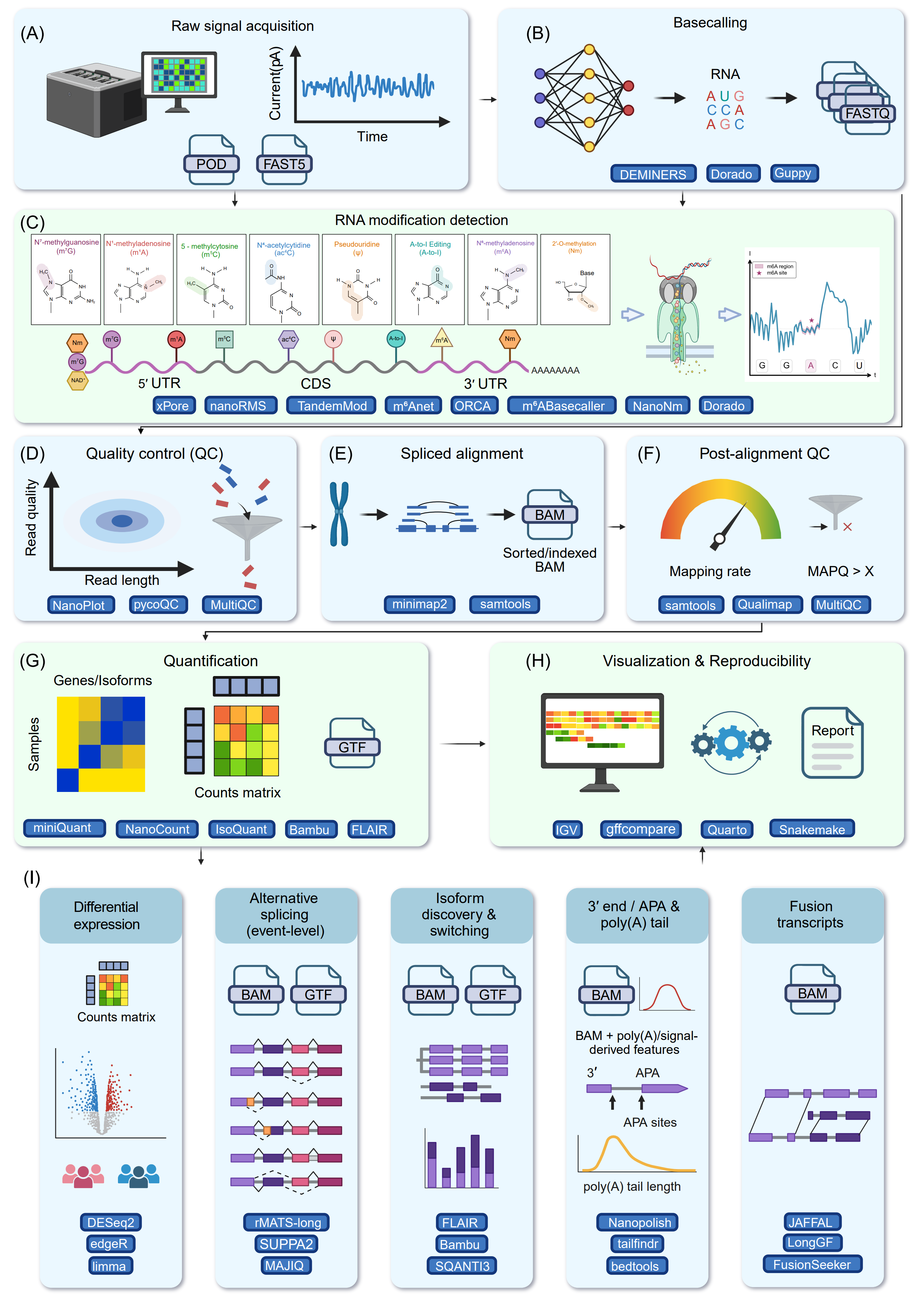
Figure 6. End-to-end computational workflow for Oxford Nanopore DRS data analysis and downstream applications. Schematic representation of a typical DRS bioinformatics pipeline, illustrating the progression from raw data to biological interpretation, with corresponding bioinformatics tools for each analytical phase highlighted in blue boxes. (A) Acquisition and storing of raw ionic current signals in native nanopore sequencing file formats (POD/FAST5). (B) Basecalling transforms raw ionic current signals into nucleotide sequences formatted in standard FASTQ. (C) Direct identification of RNA modifications from signal-level characteristics spanning essential transcript regions (5′ UTR, CDS, and 3′ UTR), encompassing prevalent epigenetic markers and editing occurrences (e.g., m⁶A, m⁵C, Ψ, ac⁴C, m¹A, m⁷G, A-to-I, Nm). (D) Pre-alignment quality control (QC) to evaluate fundamental sequencing variables such as read length and read quality. (E) Spliced alignment of DRS reads to the reference genome/transcriptome, resulting in aligned reads processed into sorted and indexed BAM files. (F) Post-alignment quality control to summarize genomic mapping parameters, including overall mapping rate and distributions of MAPQ scores. (G) Transcript and gene-level quantification informed by standard gene annotation files (GTF), producing a gene/isoform counts matrix for subsequent statistical analysis. (H) Data visualization and reproducible scientific reporting, encompassing genome-browser-based examination of transcriptome characteristics and organized workflow management for analytical reproducibility. (I) Diverse downstream biological analyses facilitated by long-read DRS data encompass transcript differential expression analysis, event-level alternative splicing analysis, de novo isoform discovery, isoform switching analysis, 3′ end usage/alternative polyadenylation analysis, poly(A) tail length estimation, and fusion transcript detection from full-length RNA reads.

The analysis begins with basecalling, where raw ionic current signals are converted into nucleotide sequences (Figure 6B). Basecallers utilize a variety of architectures, including Hidden Markov Model (HMM) [490], [491], convolutional neural networks (CNNs) [492], recurrent neural networks (RNNs) [493], attention mechanisms [494], and transformer models [495], to interpret current signals [496], [497].

Following basecalling, nanopore DRS enables a wide spectrum of RNA-centric analyses, with RNA modification profiling representing one of its most important capabilities (Figure 6C). Unlike short-read sequencing approaches that rely on RT or chemical conversion, nanopore sequencing directly measures ionic current disruptions as native RNA molecules pass through the pore [56], [388], [498]. Chemical modifications on nucleotides alter the local current signal and basecalling behavior, generating characteristic deviations that can be computationally modeled to infer modified bases at single-molecule resolution [177], [183], [188], [499]. Recent advances in modification-aware basecalling frameworks now support transcriptome-wide detection of several prevalent modifications, including m6A, A-to-I, Ψ, and m5C, while preserving full-length transcript context [372], [500].

In addition, systematic read-level quality control (QC) is performed to assess sequencing performance and curate the dataset prior to downstream analysis. QC procedures typically include evaluation of read length distributions and removal of low-quality or excessively short reads (Figure 6D). NanoPlot [501] provides comprehensive visualization and summary statistics of read length distributions, quality scores, throughput, and channel activity from FASTQ or sequencing summary files. Fastplong [502] provides an integrated framework that combines QC reporting, flexible read filtering, adaptor trimming, and poly(A) tail removal, features particularly relevant for DRS and full-length transcriptome analyses. In practice, visualization tools and filtering utilities are often used together to ensure standardized, reproducible, and high-quality ONT data processing.

Beyond RNA modifications, Nanopore DRS also enables downstream transcript quantification and structural characterization. Full-length reads are mapped to their genomic or transcriptome origin using long-read-aware spliced aligners (Figure 6E). Optionally, post-alignment quality control can be performed to assess mapping accuracy, splice junction support, read completeness, and coverage uniformity, thereby minimizing artifacts and false-positive transcript models (Figure 6F). Based on read alignments, transcript reconstruction frameworks define full-length transcript isoforms, refine transcript boundaries, and update gene annotations [210], followed by isoform- and gene-level expression quantification to enable differential expression analysis across conditions (Figure 6G) [86]. Representative alignment patterns and transcript architectures can be further visualized in genome browsers (Figure 6H). Beyond expression profiling, nanopore DRS supports comprehensive characterization of RNA processing and structural diversity, including detection of AS patterns, identification of novel splice junctions, estimation of poly(A) tail length and APA sites, mapping of transcription starts and termination sites, and discovery of fusion transcripts and noncoding RNAs (Figure 6I). Together, these capabilities provide a unified, transcript-resolved view of RNA processing and post-transcriptional regulation. Importantly, because nanopore DRS sequences full-length native RNA molecules at single-molecule resolution, these diverse features can be measured concurrently on the same RNA strand, enabling direct investigation of how RNA modifications are coordinated with splicing patterns [503], poly(A) tail dynamics, and transcript stability [60], and thereby offering an integrated perspective on post-transcriptional gene regulation that is not achievable with fragmented or ensemble-based sequencing approaches.

Basecalling

Basecalling is the computational process that translates raw nanopore ionic current signals into nucleotide sequences by inferring base sequence underlying the measured electrical signal. A variety of basecalling tools are available for DRS [334], [504], [505], [506]. Guppy is an earlier ONT basecaller, developed in C++ as a closed-source replacement for Albacore, and in the context of DRS it supports only the SQK-RNA002 chemistry, making it increasingly outdated as new chemistries emerge. Dorado is ONT’s current flagship high‑performance basecaller, designed to convert raw nanopore electrical signals into DNA or RNA sequences using optimized deep‑learning architectures. Compared to Guppy, Dorado offers substantial improvements in basecalling accuracy and throughput, supports multiple flow cells and chemistries including SQK-RNA002 and SQK-RNA004, and features a modular design that enables advanced functionalities such as modified basecalling and duplex calling. Unlike Guppy and Dorado, which are primarily optimized for inference, Bonito offers greater flexibility for users who wish to retrain or fine‑tune basecalling models on custom datasets, though this comes at the cost of requiring deeper computational expertise and more extensive GPU resources.

Among open‑source community tools, RODAN [504] was the first to introduce an EfficientNet‑style pure convolutional architecture for RNA basecalling. DEMINERS [334] is a comprehensive RNA-omics toolkit that extends beyond basecalling to include barcode demultiplexing, direct pathogen assembly, and clinical metagenomic analysis. GCRTcall [505] adopts a fundamentally different strategy by applying the Conformer architecture from speech recognition to nanopore RNA signal processing. Coral [506] represents one of the most recent advances in RNA basecalling and implements an extreme form of dual‑context “signal-sequence” modeling.

In summary, the selection of a nanopore RNA basecalling tool should be guided by specific application needs. Dorado (for SQK-RNA004) or Guppy (for SQK-RNA002) is appropriate for plug‑and‑play usage and maximum compatibility. For early SQK-RNA002 datasets with sufficient computational resources, Coral currently provides the highest accuracy, while DEMINERS is optimal when integrated basecalling and barcode demultiplexing are required. With the increasing adoption of SQK-RNA004 chemistry and improved accessibility of GPU resources, nanopore RNA basecalling has effectively entered the “99% accuracy era”. For users prioritizing processing speed, stability, and ecosystem compatibility, Dorado remains the preferred choice. In contrast, most open‑source models are implemented in Python and lack industrial‑grade deployment optimization, resulting in comparatively lower decoding throughput.

RNA modifications detection tools

DRS enables the direct study of RNA chemical modifications by reading individual RNA molecules in real time. As an RNA strand ranslocate through a nanopore, chemical modifications create distinct perturbations in the ionic current signal [460]. By decoding these signal changes, researchers can identify modification sites at the single-molecule level. Over the past few years, a growing suite of computational tools has been developed to detect and map these RNA modifications from DRS data [334], [504], [505], [506]. An overview of tools for detecting RNA modifications based on DRS is summarized in Table S3. These methods can be broadly classified into three categories based on their underlying principles, including statistical comparison of nanopore sequence or signal features, machine‑learning models trained on signal features, and modification-aware basecalling approaches.

Statistical-based approaches represent the earliest and most conceptually straightforward class and can be further subdivided into two major categories. The first category comprises statistical, signal-level comparison frameworks that treat RNA modifications as distributional shifts in the raw current signal. These methods typically operate after “resquiggling” (realigning signal events to reference positions) and then test whether current intensity or dwell-time distributions differ between experimental conditions, such as modified versus unmodified samples or wild‑type versus knockout datasets. Early pipelines such as Tombo [507] established the basic workflow of signal alignment and per-site hypothesis testing, while comparative frameworks such as Nanocompore [34] formalized differential modification detection by contrasting signal distributions across conditions using Kolmogorov-Smirnov tests or bivariate Gaussian mixture models. More recent probabilistic approaches such as xPore [185] model per-site signals as mixtures of modified and unmodified states via a Bayesian framework, enabling estimation of modification rates (stoichiometry) and differential modification across samples, often without requiring a perfectly “unmodified” control. Related single-molecule quantification frameworks, exemplified by nanoRMS [186], extend distributional comparison to per-read clustering, enabling stoichiometry estimates and heterogeneity analysis at the molecule level. The primary strength of statistical signal comparison methods lies in their discovery potential, as they are modification-agnostic and do not require prior knowledge of modification signatures; however, they typically demand deep sequencing coverage, are sensitive to signal alignment accuracy, and cannot distinguish between different modification types that produce similar current perturbations.

The second category leverages basecalling error signatures as proxies for RNA modification. In this paradigm, modifications are inferred from systematic mismatches, indels, trace deviations, or quality-score perturbations at specific sites. Tools such as DiffErr [52] and DRUMMER [387] exemplify differential error-based detection for m6A, typically by comparing wild-type to writer knockout or knockdown conditions and identifying positions where error profiles shift reproducibly. DRUMMER includes a specific m6A mode that reports the distance to the nearest AC dinucleotide and the 5‑nt sequence motif centered on that motif (NNACN). EpiNano [56] extended this logic by building supervised classifiers on engineered error features derived from synthetic constructs, demonstrating that basecaller errors can carry reproducible modification information even without explicit signal modeling. EpiNano is specifically trained and applied within RRACH motifs (the known m6A consensus sequence), as its analysis and predictions are restricted to this motif context. Similarly, NanoPsiPy [508] exploits the unique U-to-C mismatch pattern characteristic of Ψ in DRS data. ELIGOS [173] uses statistical models of systematic basecalling errors to detect various RNA modifications at single-base resolution without requiring machine learning. Error-driven strategies are computationally efficient and can perform well for modifications with strong, consistent basecaller error footprints; their main limitations are tight coupling to specific basecaller versions and chemistry platforms, as well as reduced robustness for modifications that do not produce distinct error signatures.

Machine learning-based approaches constitute the largest group and infer RNA modifications directly from nanopore signal features. These methods employ supervised or weakly supervised machine learning approaches that operate on engineered features derived from either raw current signals, basecalling traces, alignment context, or combinations thereof. These models use either machine learning models such as support vector machines (SVM), random forests, gradient boosting, or deep learning architectures such as BiLSTMs, ResNets, attentions, and transformers to map feature vectors around candidate sites to modification probabilities. For m6A, tools such as MINES [176], which employs a random forest classifier, and nanom6A [172],which utilizes an XGBoost model, combine current-derived features with motif or k-mer constraints and train classifiers using sites supported by orthogonal assays or synthetic standards. m6Anet [175] employs a deep learning framework based on multiple-instance learning (MIL), enabling site-level m6A detection and stoichiometry estimation without requiring read-level labels or matched knockout controls. RedNano [509] integrates raw signal features with base-calling error profiles through a residual neural network, achieving strong generalization across phylogenetically distant species. Xron [58] incorporates a convolutional recurrent neural network combined with HMM to perform methylation-aware basecalling, allowing simultaneous sequence decoding and m6A identification from the same signal stream. Models like pum6a [405] and SingleMod [179] use techniques such as positive-unlabeled learning and attention mechanisms to deduce modification states from individual reads, even with incomplete training data.

For other marks, analogous feature-engineered and learning-based strategies have been extended beyond m6A to encompass a broader spectrum of epitranscriptomic modifications. For m5C, deep learning frameworks including CHEUI [182], TandemMod [177], and modCnet [188] combine raw signal features with neural architectures to enable transcriptome-wide and single-molecule resolution profiling. For Ψ, a diverse set of tools has emerged that leverage both signal distortions and base-calling discrepancies. Methods such as NanoPsu [57], Penguin [187], and IndoC [510] use supervised or semi-supervised machine learning on signal and alignment-derived features. More recent deep learning models, NanoSPA [183] and NanoMUD [499], further enable high-resolution and, in some cases, multi-mark detection involving Ψ and related derivatives such as m1Ψ. For A-to-I RNA editing, signal-aware deep learning approaches such as Dinopore [511] directly model ionic current traces using convolutional neural networks, while DENA [174] and related frameworks demonstrate that recurrent architectures trained on native RNA can capture editing-associated signal perturbations without reliance on genome-based SNP filtering. Complementary anomaly-detection strategies, such as iForest [512], instead exploit systematic base-calling deviations to distinguish C-to-U editing events from sequencing noise. Detection of Nm has similarly benefited from supervised models that integrate signal statistics and k-mer context, including Nm-Nano:ref:[513] <ref513> and NanoNm [514], which apply ensemble machine learning to achieve single-nucleotide resolution mapping. Specifically, NanoNm has validated its Nm detection method across multiple species and identified FBL-associated or Nm-deficient sites in both rRNA and mRNA. A key challenge in detecting these modifications is their low abundance relative to m6A [515], creating severe class imbalance in machine learning models. This often leads to increased false positives when optimizing for sensitivity, while stricter thresholds to improve precision risk missing true modification sites, making accurate detection inherently difficult.

Beyond single-modification tools, a growing number of integrative systems aim to characterize multiple RNA modification types simultaneously from the same dataset. Frameworks such as TandemMod [177], modCnet [188], NanoRL [516], DirectRM [180], ORCA [503], and CircRM [517] employ multi-label deep learning or transfer learning strategies to profile diverse combinations of m6A, m5C, Ψ, m1A, hm5C, ac4C, and related marks across transcript classes. Among them, 6 tools including m6Anet, singleMod, TandemMod, epiNano, NanoSPA, and Dinopore were retrained for simultaneous detecting multiple types of RNA modifications from both SQK-RNA002 and SQK-RNA004 data [518]. These multi-mark approaches offer the advantage of maximizing information extraction from limited sample material, but they also face greater computational complexity and require carefully curated training data with ground-truth annotations for multiple modification types.

Another category comprises basecaller-integrated frameworks that streamline RNA modification detection by embedding it directly into the sequence decoding process. Rather than treating modification calling as a separate downstream analysis step, these approaches infer per-read modification probabilities during basecalling or immediately thereafter, typically by jointly modeling nucleotide sequence context and modification-induced perturbations in the ionic current signal. Representative tools in this category include Dorado [500], Remora [519], m6Abasecaller [372], mAFiA [181], and IL-AD [520], all of which employ neural network architectures trained to simultaneously decode canonical sequence information and modification signatures from raw or basecaller-derived signal features. For example, m6ABasecaller incorporates m6A prediction directly into the basecalling workflow, enabling real-time, single-molecule detection without requiring matched control samples or post hoc signal processing. Similarly, Dorado, the current basecaller developed by ONT, provides pretrained models for multiple RNA modifications, allowing concurrent sequence reconstruction and multitype modification inference within a unified computational pipeline. A notable advantage of basecaller-integrated frameworks is their streamlined, one‑step workflow and reduced need for downstream post‑processing; however, they offer less flexibility for users who wish to customize feature engineering or apply alternative model architectures to specific research questions.

In practice, for RNA002 data, m6Anet is recommended for m6A detection due to its balanced precision-recall and strong wild-type versus knockout discrimination [162], [518]. For RNA004 data, Dorado is the default performer across m6A, m5C, Ψ, and A-to-I, achieving an area under the receiver operating characteristic curve (AUROC) of 0.9. Retrained SingleMod, TandemMod, EpiNano, NanoSPA, and DinoPore can serve as alternative options for detecting these RNA modifications. Notably, while m6A remains the most accurately detected modification, non-m6A tools in both chemistries require substantial improvement in precision-recall balance and biological validity [518].

In summary, RNA modification detection tools for nanopore DRS have evolved from statistical signal comparison and error-based inference to advanced machine learning and basecaller-integrated frameworks. These approaches differ in their assumptions, data requirements, and resolution, ranging from modification-agnostic differential analyses to single-molecule, multi-mark profiling. While learning-based and integrated basecalling models offer improved sensitivity and scalability, careful benchmarking, model selection, and validation remain essential to ensure robust and biologically meaningful interpretation.

Training datasets and resources for building nanopore RNA modification detection models

The development of accurate computational models for RNA modification detection from nanopore DRS data critically depends on the availability of high-quality training datasets with reliable ground truth labels. Because nanopore signals are influenced by both sequence context and chemical modifications, training data must be carefully designed to disentangle these factors and expose models to diverse k-mer environments and stoichiometries.

One major source of training data comes from IVT RNA with site-specific modifications. In this approach, synthetic RNA molecules are generated in which a defined fraction or all copies of a particular nucleotide at known positions carry a specific modification. By sequencing both modified and unmodified versions of the same RNA, researchers obtain paired datasets that differ only in chemical state, providing clean labels for supervised learning. Such datasets are particularly valuable for learning modification-specific signal signatures and for calibrating models to estimate modification stoichiometry. Representative examples include the widely used Curlcake and ELIGOS synthetic RNA constructs [56], in which long designer sequences were computationally generated to contain all possible 5-mer contexts while minimizing RNA secondary structure. These sequences were split into manageable fragments, transcribed in vitro, and selectively synthesized with modified nucleotides such as m6A incorporated during transcription. A second important class of IVT training substrates consists of systematically designed short templates targeting defined 5-mer contexts [173]. In these libraries, synthetic DNA templates are engineered such that a central 5-mer contains one or more occurrences of a specific base, which is replaced during transcription with a modified nucleotide (e.g., m6A, m1A, m5C, hm5C, f5C, Ψ, m7G, or inosine). Flanking sequences are designed to avoid the same base, ensuring that the modification signal can be attributed unambiguously to the targeted positions. However, IVT systems often lack the sequence diversity of native transcriptomes, which can limit model generalization if used alone. To address this limitation, Wu et al. constructed an in vitro epitranscriptome training resource (IVET) [177], [188] by performing IVT on a large rice cDNA library, generating thousands of transcripts that collectively span a broad spectrum of natural sequence contexts.

However, despite their value as controlled training resources, IVT-based modification datasets also have important limitations. In many IVT designs, the canonical nucleotide triphosphate is completely replaced with a modified analog. As a result, every occurrence of that base in the transcript becomes modified, rather than only a subset of biologically selected positions. This produces transcripts with unrealistically high and uniform modification density, which differs substantially from native RNA.

Another complementary strategy uses native biological samples combined with orthogonal experimental assays to provide site-level labels for model training and evaluation. In this framework, transcriptome-wide maps generated by biochemical methods combining with short reads sequencing are used as reference annotations to supervise or benchmark nanopore-based predictions. For example, miCLIP enables near-single-nucleotide mapping of m6A through antibody crosslink, induced mutation signatures [34], while m6A-REF-seq and related endoribonuclease-based approaches identify m6A sites by exploiting methylation-sensitive cleavage patterns [166]. For m5C, RNA bisulfite sequencing provides base-resolution detection by selectively converting unmodified cytidines [182]. A number of well‑constructed databases such as RMBase v3.0 [521], RM2Target v2.0 [522], MeT-DB v2.0 [523], REPIC [524], and PRMD [525], aggregating RNA modifications from diverse epitranscriptome sequencing datasets across multiple species, provide an abundant resource for training models on specific RNA modification types.

Nevertheless, these reference maps have important limitations that must be considered when used as ground truth. First, most orthogonal assays are population-averaged and do not preserve single-molecule information, whereas nanopore sequencing measures modification signals at the level of individual RNA molecules. As a result, discrepancies may arise between site-level enrichment detected by biochemical methods and per-read heterogeneity observed in nanopore data. Second, many assays rely on antibody enrichment or chemical reactivity, which can introduce biases related to antibody specificity, cross-reactivity, or incomplete derivatization. For instance, miCLIP can preferentially detect high-stoichiometry sites and may miss lowly modified or structurally occluded positions, while bisulfite conversion efficiency in RNA can be affected by secondary structure, leading to false negatives or incomplete conversion [526]. In addition, RNA modifications are often dynamic and context-dependent, varying across cell types, developmental stages, or environmental conditions [527].

Despite these caveats, orthogonal assays remain an essential resource for nanopore model development. When carefully matched in biological context and combined with IVT-based synthetic controls and genetic perturbation datasets, they provide critical external validation and help anchor computational predictions to experimentally supported modification sites. A practical strategy for robust model development is to combine multiple data sources, using IVT datasets to learn modification-specific signal signatures and orthogonal assays to provide biological context and validation, thereby leveraging the complementary strengths of each approach while mitigating their individual limitations.

Isoform identification and quantification

Nanopore DRS provides full-length, single-molecule reads that span entire transcripts, allowing direct observation of exon connectivity, AS sites, TSS, and PAS. Because sequencing occurs on native RNA rather than cDNA, DRS avoids RT and PCR biases and preserves transcript structure together with molecular features such as RNA modifications and poly(A) tails [528]. This makes DRS particularly powerful for isoform-resolved transcriptome analysis, where accurate reconstruction of complete transcript structures is essential.

Several specialized computational tools have been developed to reconstruct and quantify isoforms from long-read RNA data (Table S4). IsoQuant [90] uses an intron-graph framework to model splice junction connectivity and performs well in balancing sensitivity and precision across diverse transcript structures. However, its performance may be affected when reads are highly truncated at both ends. StringTie2 [89], originally developed for short reads, includes a long-read mode that builds splice graphs from aligned reads to assemble transcript models and estimate abundances. StringTie2 demonstrates high computational efficiency and strong sensitivity across datasets, though its performance can be affected by high sequencing depth or read truncation at both ends. Bambu [91] applies statistical modeling and adaptive thresholds to control false discovery while enabling novel isoform detection, making it particularly suitable when a reference annotation is available but incomplete. Bambu heavily relies on splice junctions for transcript discovery, which limits its ability to identify transcripts that differ only in alternative start or end sites, and its default exclusion of subset transcripts may lead to missed valid isoforms while biasing quantification toward non‑subset transcripts [91]. Additional graph- and clustering-based approaches have also been proposed, including Freddie [529], which detects AS patterns through read clustering without relying on existing annotations, and ESPRESSO [530], which emphasizes accurate splice junction correction and isoform quantification from long-read RNA-seq data despite its substantial memory consumption.

Other frameworks emphasize correction and filtering of long-read-specific artifacts. FLAIR [88] integrates splice-junction correction and can incorporate short-read evidence to refine isoform boundaries. TALON [531] focuses on annotation consistency across replicates and is often used in multi-sample studies to track known and novel transcripts. FLAME [532] models read truncation and transcript length biases, which is helpful for distinguishing true isoforms from partial reads. SQANTI3 [533] provides a comprehensive quality-control and classification framework for long-read transcript models, enabling systematic assessment of splice junction validity, structural novelty, and artifact enrichment relative to reference annotations. Recently developed tools such as Longcell [534] further extend isoform-resolved analysis by integrating long-read transcript structures with single-cell resolution. Benchmarking studies using spike-in controls and nanopore datasets show that graph-based methods such as IsoQuant and StringTie2 generally achieve strong sensitivity for complex genes, while model-based approaches like Bambu can better control false positives when discovering new isoforms [216], [535].

Using these tools, DRS data enable direct identification of diverse isoform features, including exon skipping, intron retention, alternative donor and acceptor sites, promoter switching, and alternative last exons. Because each read represents a single RNA molecule, isoform abundance can be directly estimated from read counts without fragment reconstruction, while isoform identity can be analyzed together with RNA modification profiles, poly(A) tail length, and transcriptional termination variability. This enables integrated investigation of transcript architecture, RNA processing, and post-transcriptional regulation at single-molecule resolution [52], [86], [189], [328].

Despite these advantages, isoform reconstruction from DRS remains sensitive to long-read-specific technical factors. Residual basecalling errors, incomplete 5′ end coverage, and alignment ambiguity in repetitive regions can lead to false splice junctions or truncated isoforms [35], [81]. Increasing sequencing depth improves detection of low-abundance transcripts but can also elevate false-positive isoforms if filtering is not applied [84]. Therefore, practical analyses usually apply minimum junction support thresholds, transcript read support filters, and optional hybrid correction using srRNA-seq data [91].

In a typical DRS isoform analysis workflow, raw POD5 signal files are first basecalled with neural network models such as Dorado from ONT. The resulting reads are aligned to a reference genome using splice-aware long-read aligners such as Minimap2, configured for native RNA. Aligned reads are then processed by long-read transcriptome assemblers to collapse reads into isoform models and quantify expression. Subsequent filtering, annotation comparison, and differential isoform analyses produce a high-confidence, isoform-resolved view of the transcriptome. Benchmarking analysis revealed that IsoQuant consistently achieved the highest precision and sensitivity across most simulation scenarios, sequins datasets, and experimental datasets [216]. It performed particularly well in complex settings such as high isoform diversity and incomplete annotations, and it maintained stable performance across varying sequencing depths and error rates. Therefore, IsoQuant is recommended for accurate isoform detection in long-read RNA sequencing data.

Poly(A) and APA analysis

In most eukaryotes, the poly(A) tail is a non‑templated adenosine tract at the mRNA 3′ end that contributes to mRNA maturation and export and shapes cytoplasmic mRNA stability [385], [536]. Historically, transcriptome‑wide poly(A) profiling has relied on RT and PCR‑based methods, which can introduce amplification‑driven distortions and decouple tail features from the native RNA molecules being inferred [226]. Nanopore DRS addresses these limitations by sequencing native RNA molecules directly, enabling single‑molecule linkage between isoform identity and poly(A) tail information within the same read [35].

In ONT DRS, RNA molecules are physically translocated through the nanopore in the 3′‑to‑5′ direction, while basecalling software reports sequences in the 5′‑to‑3′ orientation, placing the poly(A) segment at a stereotyped location in the raw signal [35], [228]. Consequently, most poly(A) length estimators operate at the signal level, segmenting the low‑variance poly(A) current plateau, quantifying its duration in raw samples, and converting this value to nucleotides using a per‑read estimate of the translocation rate, typically expressed as samples per nucleotide [9], [35], [226], [228], [229], [492].

Several tools have become widely used for poly(A) localization and length estimation from DRS data, differing mainly in how they segment the signal and normalize for read‑specific kinetics. Nanopolish [491] implements a segmentation HMM and uses Viterbi decoding to infer region boundaries that include the poly(A) segment, estimating tail length from the inferred poly(A) duration and a read‑specific rate [35]. tailfindr provides an alignment‑free alternative that uses smoothed signal heuristics to locate the tail boundary and derives per‑read normalization from basecaller‑derived information [228]. Benchmarking against synthetic RNA standards demonstrated that tailfindr achieves high accuracy for poly(A) estimation, performing comparably to Dorado across various tail lengths [537]. However, its runtime is slower than that of Dorado and Nanopolish, and it requires basecalled FAST5 files, which adds preprocessing complexity and limits compatibility with newer sequencing workflows. BoostNano [537] employs a deep‑learning sequence‑labeling strategy to segment adapter‑ and tail‑associated regions directly from raw signal [492], [537]. BoostNano exhibits pronounced multimodal distributions and tends to overestimate very short poly(A) tails [537]. Dorado, ONT’s official basecaller, offers built‑in poly(A) and poly(T) length estimation and records the estimate as a BAM tag. It identifies a primer anchor for the tail, uses the move table to delimit the tail interval in raw signal, and converts signal span into nucleotide length [537]. Recent benchmarking using synthetic RNA standards recommended Dorado as a preferred approach due to its fast runtime and low mean error [537]. For downstream comparison and visualization, TAILcaller [538] operates directly on Dorado BAM files, whereas NanoTail provides analysis utilities focused on Nanopolish outputs [229]. Benchmarking using synthetic RNA standards (Sequins) with known poly(A) tail lengths demonstrated that nanopolish, tailfindr, Dorado, and BoostNano all recover mean tail lengths within ~12% of the ground truth, although they differ in variance, computational efficiency, and stringency of read filtering [537].

Beyond tail length measurement, nanopore DRS also supports analysis of APA. Alignment of full-length reads reveals transcript 3′ end heterogeneity, allowing identification of distinct PAS within the same gene. APALORD [539] provides an integrated pipeline that quantifies poly(A) sites usage and performs differential APA analysis between conditions, enabling proximal-distal switching to be assessed within a unified framework. LAPA [540] similarly clusters transcript termini into PAS peaks and estimates site usage, offering a flexible PAS‑calling approach applicable to long‑read datasets, including DRS, although differential testing is typically conducted downstream according to study‑specific designs.

In viral and other compact genomes, end‑site discovery tools are often used to define TSS and cleavage and polyadenylation sites (CPAS) catalogs that serve as proxies for PAS in APA‑like quantification. NAGATA [210] identifies CPAS by clustering enriched DRS 3′ ends while applying filters to reduce artifactual termini, whereas LoRTIA [541] detects statistically enriched transcript end sites from long‑read alignments using end‑enrichment signals and alignment features such as soft clipping. These approaches are frequently employed to reconstruct complex termination landscapes and can be readily extended to comparative APA analyses by quantifying reads assigned to alternative end‑site clusters across samples.

Most DRS studies still infer APA indirectly through isoform reconstruction followed by boundary standardization. DRS‑capable transcriptome analysis tools (IsoQuant [90], FLAIR [88], FLAMES [383], Bambu [91], TALON [531]) generate quantified transcript isoforms whose 3′ ends can be clustered on a per‑gene basis into PAS and compared across conditions. IsoTools [542] and IsoTools2 [543] further incorporate gene‑wise peak calling of 3′ ends to define candidate PAS within a long‑read transcriptome analysis framework, producing PAS catalogs that can be quantified across samples, although differential APA testing is typically performed downstream.

In addition to 3′ end analysis, transcript boundary definition at the 5′ end is conceptually related but technically more challenging in DRS data. Nanopore DRS enables observation of native RNA molecules but introduces systematic 5′ truncation due to incomplete capture of transcript termini during sequencing, which complicates TSS detection. NAGATA [210] and LoRTIA [544] identify TSS by analyzing the genomic distribution of read start positions in aligned DRS reads. Other approaches, such as TranscriptomeReconstructoR [545] and Telos [546], refine transcript boundaries using existing transcript annotations or external datasets, including cap-associated short-read data, rather than performing de novo TSS discovery from DRS reads.

Importantly, poly(A) tail length and APA analyses can be integrated with other DRS-derived features at the single-molecule level. For example, tail length distributions can be examined in the context of specific isoforms, RNA modification status, or splicing patterns, enabling investigation of coordinated regulatory mechanisms that link RNA processing events. This integrative capability represents a major conceptual advance over traditional poly(A) assays, which typically measure tail length independently of transcript identity.

Nevertheless, poly(A) tail estimation and APA analysis based on nanopore DRS remain sensitive to several technical factors, including signal noise, variable RNA translocation speed through the pore, basecalling model assumptions, and RNA degradation [109], [226], [228], [481]. Very short or partially degraded poly(A) tails may be difficult to resolve accurately, and systematic differences can arise between analytical tools or sequencing chemistries. Dorado, integrated directly into ONT’s basecalling workflow, is recommended for most applications due to its fast runtime, low mean error, and conservative filtering. For scenarios where accuracy across highly variable tail lengths is prioritized over speed, such as low-throughput studies, tailfindr serves as a strong alternative. In addition, internal priming at A-rich genomic regions can mimic genuine cleavage sites, while alignment artifacts near transcript ends may shift apparent polyadenylation positions, making cleavage site clustering and filtering essential [52]. Consequently, best practices for DRS-based poly(A) and APA analysis include stringent quality control and filtering of low-confidence reads, removal of internal priming artifacts, comparison across biological replicates, and emphasis on relative or distributional differences rather than absolute tail length estimates when interpreting biological trends.

Advanced analysis and visualizations

Existing DRS data analysis tools are often functionally fragmented and tend to focus on a single analysis layer, which creates a practical barrier for users without a strong bioinformatics background. Based on published DRS studies and common needs in real-world projects, we summarized a set of advanced but frequently used analysis and visualization patterns for DRS data (Figure 7), and we provide the corresponding visualization example and code (https://zhangtianyuan666.github.io/DRS_doc). These visualization templates cover multiple layers of DRS analysis, including AS, APA, poly(A) tail length, RNA modifications, transcript structural categories, functional enrichment, and differential expression. They are intended to facilitate rapid construction of customized DRS analysis workflows tailored to specific biological questions. At the AS level, our example generates sashimi plots that summarize exon coverage and splice junction usage of representative genes across conditions (Figure 7A). UpSet plots further quantify how many transcripts are affected by each splicing category and by their overlaps (Figure 7B), helping to pinpoint condition-dependent and co-occurring splicing patterns.

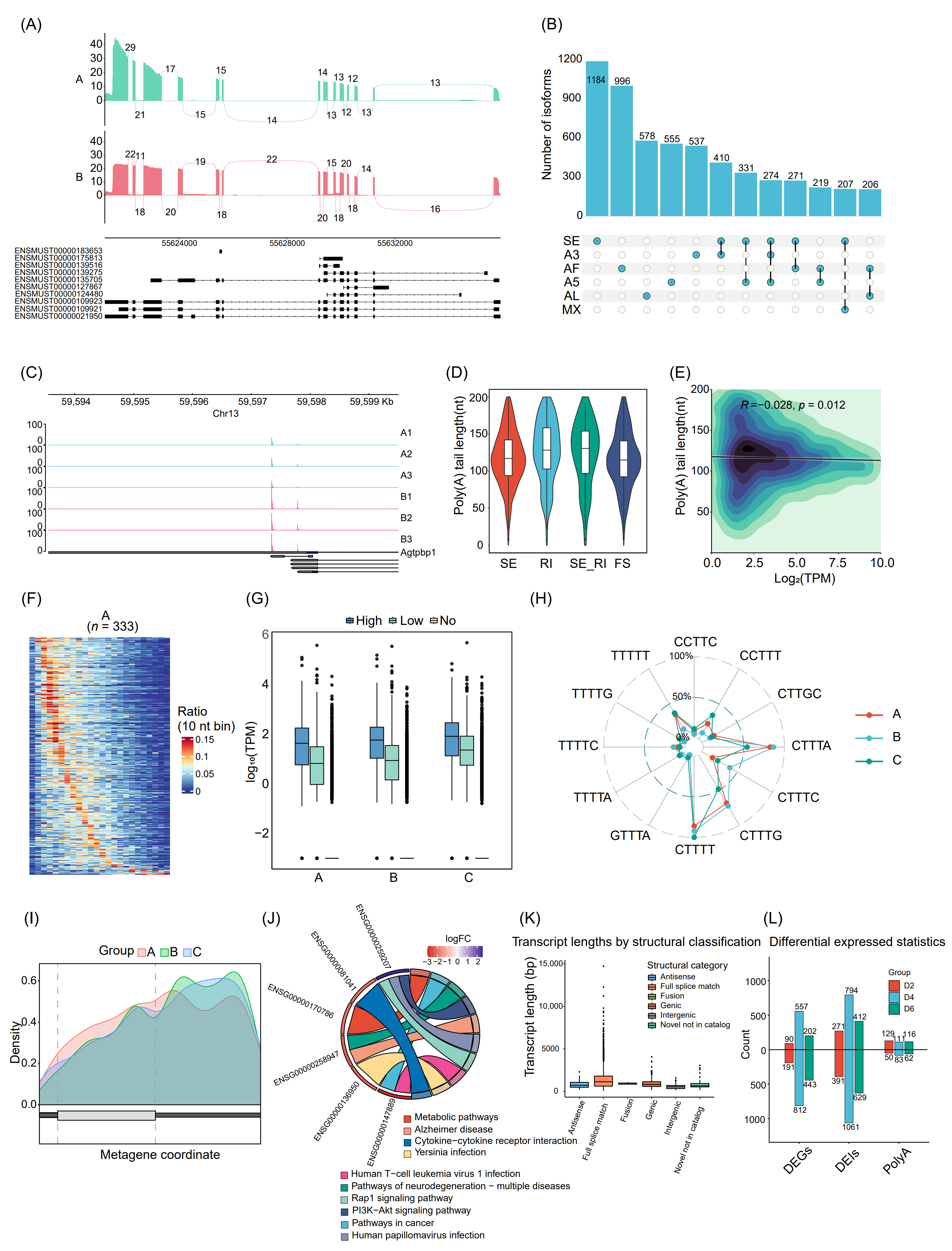
Figure 7. Representative high level analytical visualizations commonly used in DRS studies. (A) Visualization of alternative splicing and transcript coverage using ggsashimi. Sashimi plot generated with ggsashimi showing exon coverage and splice junction usage for a representative gene under two conditions (top, green; bottom, red), with annotated transcript isoforms displayed below. (B) Combinatorial patterns of AS isoforms. UpSet plot showing the number of isoforms involving different alternative splicing types and their combinations; SE: Skipped Exon; A3: Alternative 3′ splice site; A5: Alternative 5′ splice site; AF: Alternative First exon; AL: Alternative Last exon; MX: Mutually Exclusive exons. (C) IGV visualization of alternative polyadenylation (APA) at a representative gene revealed by DRS data. Genome browser view in IGV showing poly(A) site-associated read coverage for multiple samples across the 3′ region of an APA gene, together with annotated transcript isoforms. (D) Poly(A) tail length distributions associated with distinct AS event types. skipped exon (SE), retained intron (RI), combined skipped exon/retained intron events (SE_RI) and frameshift associated events (FS). (E) Two dimensional density plot showing the association transcript abundance and poly(A) tail length. The x axis represents transcript abundance as Log2(TPM), and the y axis shows poly(A) tail length (nt). Color intensity indicates the density of data points. (F) For each group (example shown for group A, n = 333 transcripts), the x axis represents poly(A) tail length from 10 to 250 nt (25 bins of 10 nt), and each row corresponds to one transcript, with color indicating the proportion of reads for that transcript in each length bin. (G) Relationship between RNA methylation status and transcript expression. The x axis denotes sample groups (A, B, C), and the y axis shows transcript abundance (log10(TPM). (H) Top enriched pseudouridine (Ψ)-associated motifs across groups A, B and C. Each axis corresponds to one motif, radial values indicate its percentage occurrence , and colored lines represent groups. (I) Chord diagram linking selected genes to enriched pathways. The color scale (logFC) indicates the direction and magnitude of gene expression changes, while ribbons illustrate which genes contribute to each pathway. (J). Transcript length distributions across SQANTI3 structural transcript categories. The x axis indicates SQANTI3 structural categories, and the y axis shows transcript length. (K) Summary of differential expression and poly(A) changes across time points. Barplot showing the numbers of differentially expressed genes (DEGs), differentially edited isoforms (DEIs) and transcripts with differential poly(A) sites (PolyA) in groups d2, d4 and d6. (L) Modification profiles of Ψ site density across mRNA features in groups A, B and C. density plots show the normalized density of identified Ψ sites aligned by transcript features, spanning the 5′ UTR, CDS and 3′ UTR. The x axis represents the relative metagene coordinate from the 5′ UTR through the CDS to the 3′ UTR, and the y axis indicates Ψ site density. Curves correspond to different sample groups (A, B and C), highlighting both shared and distinct patterns of Ψ distribution along mRNAs among the three conditions.

For APA and poly(A) analyses, the example exports IGV-compatible tracks that display poly(A) read coverage at the 3′ends of APA genes together with their annotated isoforms (Figure 7C), enabling direct visual comparison of 3′-end usage between samples. Poly(A) tail length can be profiled by splicing event type (Figure 7D), and examined either globally using a two-dimensional density plot of transcript abundance (Log2(TPM)) versus tail length (Figure 7E) or at per-transcript resolution using 10-nt binned heatmaps of tail-length distributions (Figure 7F).

For RNA modification, the pipeline links modification calls to expression and sequence context. Using methylation as an example, transcripts are grouped into High-, Low-, and No- modification classes, and their expression distributions are compared across sample groups (Figure 7G) to assess how modification status relates to transcript abundance. Then, enriched sequence motifs and their group-specific frequencies are summarized with radar plots (Figure 7H), whereas modification profiles show the density of Ψ sites along 5′ UTR, CDS, and 3′ UTR (Figure 7I), revealing both shared and condition-specific patterns of Ψ localization along mRNA. At the functional and structural levels, this example provides several global overview visualizations. The chord diagram links differentially expressed genes to enriched pathways, with color encoding the direction and magnitude of expression changes (logFC) and ribbon width reflecting each gene’s contribution to individual pathways (Figure 7J), thereby highlighting key gene-pathway modules. Transcript length can be compared across SQANTI3 structural categories, which characterizes the complexity of transcript structures in the sample and their length distributions (Figure 7K). In addition, by summarizing differential statistics across time points, the barplot shows the numbers of differentially expressed genes (DEGs), differentially expressed isoforms (DEIs), and transcripts with differential poly(A) site usage (Figure 7L) Together, these example datasets and scripts lower the technical barrier for non-specialists to perform in-depth DRS analyses, accelerate the selection and combination of appropriate analysis strategies, and promote more standardized and reproducible interpretation of DRS data.